import shapefile
from shapely import Polygon

SHP_PATH = "neighborhoods_wgs84.shp"
neighborhoods = {}

with shapefile.Reader(SHP_PATH) as sf:
    for shape_rec in sf.shapeRecords():
            # shape_rec.shape.points - list of WKT points, used to construct
            #                             a shapely.Polygon
            # We are assuming Polygon here! If this file had points/lines/etc.
            # changes would be needed.
            polygon = Polygon(shape_rec.shape.points)
            # shape_rec.record contains the attributes as a list or dictionary
            # in this file record[0] contains the neighborhood name
            name = shape_rec.record[0]
            # associate polygon with name
neighborhoods[name] = polygon12 Geospatial Data
Goals
- Introduce concepts common to geospatial data.
- Explore tools for working with geospatial data in Python.
In this section we are going to look at the unique challenges that come with working with geospatial data.
After text and numeric data, geospatial data is the most common kind of data you’re likely to encounter working on a public interest or civic project.
It also gives us an opportunity to see an example of binary data formats, as well as real-world applications of interfaces and inheritance.
Geospatial Data Overview
Before we dive into how to work with geospatial data, we need to discuss the unique challenges presented by geospatial data.
Note
A set of tools and data formats used to interact with geospatial data is sometimes known as a Geographic Information System, or GIS.
Let’s look at a high resolution photograph of Lake Michigan:
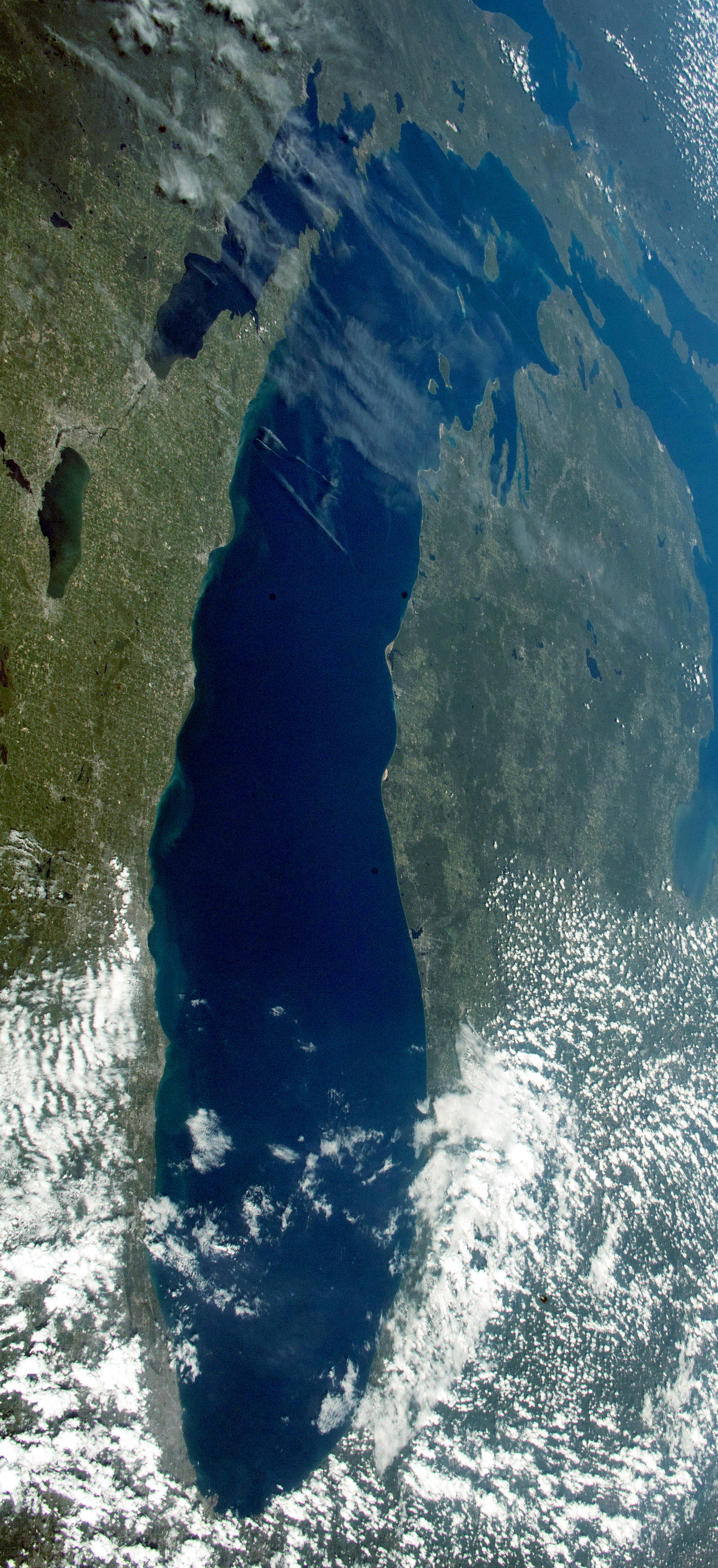
This image, like any JPG or PNG you take with your phone’s camera, is a raster image.
It is made up of individual pixels, which can be thought of as 2D matrix of (red, green, blue) values.
Reminder: Binary Files
We could store pixel data in a CSV or JSON file, but doing so wastes a lot of memory. Instead the files are stored in more efficient binary formats specially designed to compress image data based on what we know about human perception.
Text files can be opened in your editor regardless of type (.py, .md, .txt, .r, .json, .csv, .html). It is just the meaning of the characters that differs between them: < in python means “less than”, while in HTML it begins a tag.
With binary files we need to use specialized programs (MS Paint, Photoshop, QGis) and libraries (Pillow, pyshp). The meanings of the individual bits differs between them, allowing for more flexible & efficient storage of complex data.
Resolution
Natural geographic features are fractal in nature, these objects have a peculiar feature known as the coastline paradox.
In the image above, measured from space, the coast of the lake looks like a smooth curve. But, if you have walked along the actual lake, you know– it is anything but.
The more precision (shorter measure) we use to measure the coastline, the more intricate it gets, and our measurement actually gets longer.
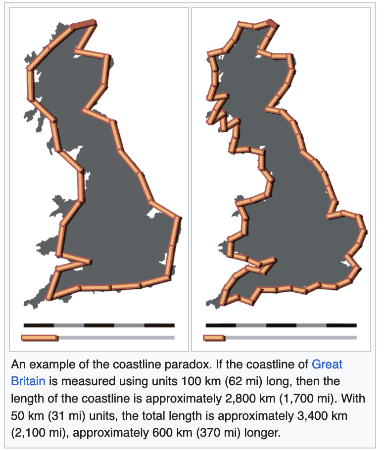 (source: Coastline Paradox on Wikipedia)
For this reason, we have to choose a resolution. This is the degree of detail that we need to include, the smallest geographic feature size we’ll be able to represent. An analysis of climate effects on large tracts of land might be fine with 100 meter resolution, while urban planning might require <1m accuracy in identifying streets or hydrants.
The higher the resolution, the more data we’ll need.
Projection
Looking at the image of the lake, it is skewed due to the angle of the photo and curvature of the earth.
Any attempt to map the surface of a sphere to a flat plane will result in distortion.
When we’re working with geospatial data we want to be able to work in (x, y) coordinates.
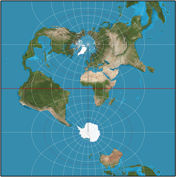
What’s wrong with this picture?
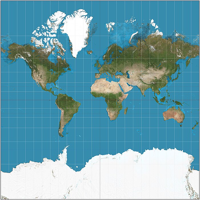 Mercator Projection, Wikipedia
Africa is 14x larger than Greenland.
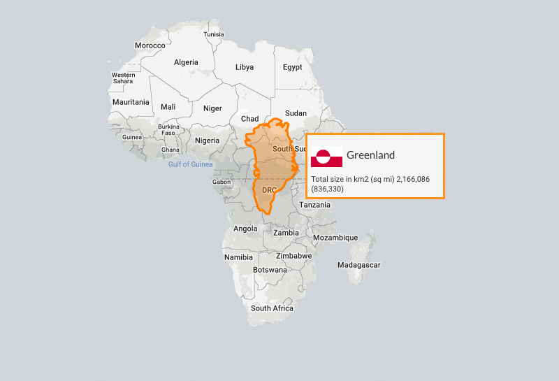 https://mortenjonassen.dk/maps/greenland-vs-africa-size-comparison
Vector Data
It turns out that for the most common applications of geospatial data, raster formats are not ideal.
The amount of data required and the need to adjust resolutions & projections, lead to vector formats being much more useful.
Instead of storing individual pixels associated with colors, these formats store geometries which can optionally be associated with features.
| Raster | Vector | |
|---|---|---|
| Pros | Efficient for continuous surfaces (can sample any point) | Arbitrary precision; Ease of calculation; Network efficiency |
| Cons | Limited by image resolution (sensor & storage) | Harder to create as specific relationships must be calculated and defined |
| Image Format | JPEG/PNG | SVG/PDF |
| GIS File Types | GeoTIFF/NetCDF | Shapefile/GeoJSON/Geopackage/KML |
| Example Data | Satellite imagery | - Points: cities - Lines: roads - Polygons: land parcels |
| Capture Tool | Camera | GPS |
Geometries
Geometries come in three main forms:
- Point -
(lon, lat)or(lon, lat, altitude)- example: address, tree, bus stop - Line aka LineString or Polyline - series of ordered, connected points - examples: roads, rivers
- Polygon - enclosed areas defined by a closed list of points - lakes, land parcels, county
Container Types:
- MultiPoint - example: fleet location, fire hydrants, GPS pings
- MultiLineString - example: branching transit line
- MultiPolygon - example: islands
We’ll revisit these when we discuss shapely.
Coordinate Reference Systems
These systems define the projection: what the x and y values actually mean in a given file.
Two kinds:
- Geographic Coordinate Systems - attempt to map a lon, lat to every point on Earth
- Projected Coordinate Systems - attempt to project earth’s curved surface onto a plane (as needed for drawing)
In practice, there are many implementations of each kind in common usage.
Different GCS account for local variations in earth’s curvature and different estimates for the exact size of the Earth. GPS uses WGS84, which has become the dominant GCS in use. When you see coordinates that resemble latitude & longitude, you are often (but not always) working with WGS84.
PCS are far more varied. No perfect mapping of a sphere to a Cartesian plane exists. The commonly used Mercator projection shows the limits, the distortion at the north and south poles is extreme. It has been historically favored because its accurate presentation of the United States and Europe.
PCS are often chosen based on the intended usage.
For a certain visualization one might opt for UTM, the Transverse Mercator projection, which minimizes distortion within a region via a set of guarantees.
Local governments will often publish in projections that are designed for high precision in their jurisdiction.
In the US this means using the State Plane Coordinate System. SPCS consists of 125 zones with their own system across the US. They are fine-tuned to fit the shape of each state to maximize accuracy. (Some use transverse Mercator, some use a Lambert conformal conic projection, all with different parameters.)
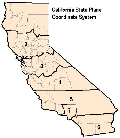 (ce: conservation.ca.gov)
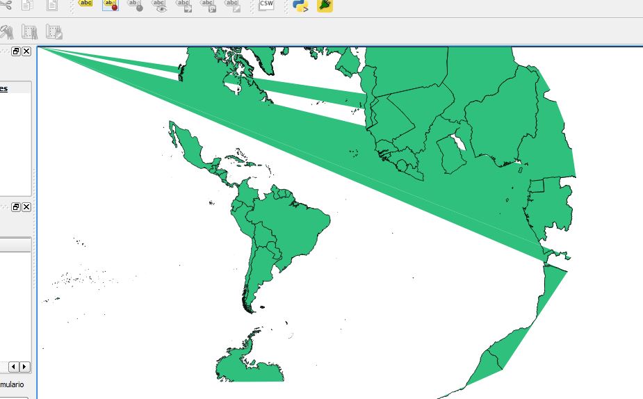
Correct Projection is Essential
Without a projection, you have a set of (x, y) coordinates with no way to connect them to reality.
What one system calls (58348, 39220) another might call (0, -10000).
Getting a coordinate system slightly wrong can lead to small but important inconsistencies or visual artifacts on your maps.
Features
Most GIS file types allow the association of features with geometries.
You can think of features as a database or spreadsheet of attributes associated with a given geometry
It might take the form:
| County Name | Population (2020) | Area (sq mi) | County Seat | Georeference |
|---|---|---|---|---|
| Cook | 5,275,541 | 1,635 | Chicago | {MULTIPOLYGON…} |
| DuPage | 932,877 | 334 | Wheaton | {MULTIPOLYGON…} |
| Lake | 714,342 | 448 | Waukegan | {MULTIPOLYGON…} |
| Will | 690,743 | 837 | Joliet | {MULTIPOLYGON…} |
| Kane | 516,522 | 524 | Geneva | {MULTIPOLYGON…} |
Formats
- shapefile - actually a bunch of files that need to live in the same directory
- .shp - geometries
- .shx - indexes for searching
- .dbf - csv-like features
- .prj - projection (CRS)
- .sbn/.sbx/.shp.xml/.cpg - additional optional files that provide more metadata and features
- GeoJSON/TopoJSON: JSON representation of features and geometries
- KML: Google XML-based format, mostly out of favor but still commonly found on GIS sites
- Geopackage: Still uncommon, sqlite based successor to shapefile.
Working with Geospatial Data
To work with geospatial data we’ll need to load the data from one of the vector formats into objects.
We are going to use pyshp aka shapefile to load the data, and shapely to work with the geometries once loaded.
The data types & operations we are using however are common to most GIS tools.
Loading a Shapefile
Geometry Objects
Shapely defines a set of geometry classes.
All of these classes inherit base behavior from shapely.Geometry:
The first three define our core geometry types, while their Multi-prefixed variants store lists of the underlying types.
This may seem unusual, why not just use a list containing Point objects?
In practice, we are going to see a lot of functions of the form p(Geometry) or f(Geometry, Geometry) and by having all of these collection classes we’ll be able use the same methods regardless of if we have one or many geometries.
GeometryCollection exists to take that idea to it’s fullest form, allowing for collections of multiple geometry types.
Example: Using Geometries
from shapely import Point

museums = [
    ("Field Museum", Point(-87.6169, 41.8663)),
    ("Art Institute of Chicago", Point(-87.6237, 41.8796)),
    ("Museum of Science and Industry", Point(-87.5830, 41.7906)),
    ("The Metropolitan Museum of Art", Point(-73.9632, 40.7794))
]

for museum, museum_point in museums:
    for neighborhood, poly in neighborhoods.items():
        if poly.contains(museum_point):
            print(museum, "is in", neighborhood)
            break
    else:
        # for-else only executes if no break did
        print(museum, "is not in Chicago!")
Field Museum is in Museum Campus
Art Institute of Chicago is in Grant Park
Museum of Science and Industry is in Jackson Park
The Metropolitan Museum of Art is not in Chicago!GIS Functions
Shapely defines many helpful functions:
measurement functions like:
area(poly_or_multipoly)- Computes polygon area.distance(a, b)- Computes Cartesian distance between two polygons.bounds(geom)- Computes the bounding box that contains the polygons.
contains(a, b)returnsTrueif the geometrybis completely withina.dwithin(a, b, distance)returnsTrueisais less thandistanceaway fromb.intersects(a, b)- returnsTrueifaandbintersect at all.
and set operations.
difference(a, b)intersection(a, b)union(a, b)
These operations are designed to work with any geometry type. This is an example of the power of the interface, instead of learning different methods for each, we can use a common set of functions that all operate on a Geometry interface.
These can also be accessed as methods on the geometries themselves (obj.contains(other)). See binary predicateshttps://shapely.readthedocs.io/en/stable/manual.html#binary-predicates) in Shapely documentation.
This means we can express common geospatial ideas in a simple way:
Where is the nearest Waffle House?
shapely.ops.nearest_points(waffle_house_multipoint, my_location)
What congressional district am I in?
in_district = [shapely.contains(poly, my_location) for poly in districts]
What attractions are near my road trip route?
# geom.buffer(dist) adds a margin around a point, line, or polygon
route_buffer = route_linestring.buffer(distance)
# find all points that fall within polygon
nearby_attractions = attractions_multipoint.intersection(route_buffer)
What part of the US is either national park or state park?
union(national_parks_mp, state_parks_mp)
How much of Illinois is fresh water?
intersection(il_boundaries, fresh_water_mp)
What parts of Cook County are not within Chicago?
difference(cook_co, chicago)
Geospatial Joins
Geospatial Joins combine two or more datasets on a condition (like overlaps or contains). This technique is used to discover overlaps between datasets, for example, to find what counties are in which cities:
joined_data = [(county, city) for county in counties for city in cities if county.geometry.intersects(city.geometry)]
A typical join between two data sets is
As you might imagine, that combined with the complexity of the underlying geometric algorithms can mean poor performance.
We can use the unique properties of geospatial data to organize the data spatially. Data structures such as Quadtrees and R-Trees can drastically speed up spatial join operations.
These are sometimes referred to as spatial indices.
Further Exploration
- pyshp
- shapely
- geopandas is an extension to
pandasthat adds Shapely types to the dataframe. While it can be helpful for small operations wherepandasis already in use– it does not support spatial indexing, and cannot be as efficient as other options.
Other Geospatial Software
The types and most operations are part of a standard known as OGC Simple Features.
This means that what you learn to do here in Python will be applicable in other GIS software and libraries.
GDAL/OGR Tools
GDAL is the C++ library that powers shapely and many other GIS applications. It provides command line tools that are invaluable if you are working with geospatial data on a regular basis. The tools can help you inspect the data, convert geometries and projections, and a lot more. There’s a helpful guide here: https://github.com/dwtkns/gdal-cheat-sheet
PostGIS
PostGIS is an extension to PostgreSQL that adds geometry types and predicates to your database. Allows querying directly from database, saving conversion and minimizing memory footprint. Like most things Postgres, one of the most solid pieces of software ever built.
QGis
QGis - 100% Free & Open Source GUI for working with GIS files.
While we won’t cover its usage in class, can be useful for inspecting/understanding the GIS data you are working with.
ArcGIS
Commercial/proprietary service. Developed by ESRI, the key commercial player in GIS for decades.
Offers cloud/server/desktop based tools.
Favored in government, large corporations, full suite is most feature complete offering around. Under increasing competition from OSS competitors which are often more lean, cutting lesser-used features and antiquated formats.